A Tiny Transformer LLM in PyTensor

Can you train a transformer language model end-to-end in PyTensor? Yes — and that is exactly what we do in this notebook. We build a small decoder-only GPT on character-level Tiny Shakespeare, train it with a hand-rolled Adam optimizer, and sample from it. Along the way we showcase what makes PyTensor distinctive for deep learning:

• pytensor.xtensor named dimensions drive multi-head attention, so the (batch, head, time, head_dim) reshape gymnastics become self-documenting code,

• a static graph you can inspect with pytensor.dprint,

• symbolic reverse-mode auto-diff via pytensor.grad,

• pytensor.shared parameter state with in-graph optimizer updates, and

• pytensor.scan for autoregressive generation — the entire sampling loop, including all forward passes and all categorical draws, runs inside a single compiled call.

The model is intentionally tiny (~100k parameters, a few thousand training steps) so the whole notebook runs on a laptop CPU in a couple of minutes.

Prepare notebook

from __future__ import annotations

import time
import urllib.request
from dataclasses import dataclass
from pathlib import Path

import matplotlib.pyplot as plt
import numpy as np

import pytensor
import pytensor.tensor as pt
import pytensor.xtensor as ptx


plt.style.use("seaborn-v0_8")

%config InlineBackend.figure_format = "retina"

rng_np = np.random.default_rng(0)
floatX = pytensor.config.floatX
print("pytensor:", pytensor.__version__, "| floatX:", floatX)

pytensor: 3.0.5+30.g1bb3ee02f | floatX: float64

Data — Tiny Shakespeare

We download Andrej Karpathy’s 1.1 MB Tiny Shakespeare corpus into a local cache directory and use a character-level vocabulary (~65 unique characters). To keep training fast on a laptop, we slice off only the first ~50,000 characters — plenty for the model to learn the shape, rhythm, and common words of Shakespearean English.

DATA_DIR = Path("data")
DATA_DIR.mkdir(parents=True, exist_ok=True)
DATA_FILE = DATA_DIR / "tinyshakespeare.txt"
DATA_URL = (
    "https://raw.githubusercontent.com/karpathy/char-rnn/"
    "master/data/tinyshakespeare/input.txt"
)

if not DATA_FILE.exists():
    print("Downloading", DATA_URL)
    urllib.request.urlretrieve(DATA_URL, DATA_FILE)

full_text = DATA_FILE.read_text()
print(f"Full corpus: {len(full_text):,} characters")

# Use a small slice so training is fast in a notebook.
text = full_text[:50_000]
print(f"Used slice : {len(text):,} characters")
print("\n--- First 200 characters ---\n")
print(text[:200])

Downloading https://raw.githubusercontent.com/karpathy/char-rnn/master/data/tinyshakespeare/input.txt
Full corpus: 1,115,394 characters
Used slice : 50,000 characters

--- First 200 characters ---

First Citizen:
Before we proceed any further, hear me speak.

All:
Speak, speak.

First Citizen:
You are all resolved rather to die than to famish?

All:
Resolved. resolved.

First Citizen:
First, you

chars = sorted(set(text))
vocab_size = len(chars)
stoi = {c: i for i, c in enumerate(chars)}
itos = {i: c for i, c in enumerate(chars)}

def encode(s: str) -> np.ndarray:
    return np.array([stoi[c] for c in s], dtype="int64")

def decode(arr: np.ndarray) -> str:
    return "".join(itos[int(i)] for i in arr)

data_ids = encode(text)
print(f"vocab_size = {vocab_size}")
print(f"first 20 ids: {data_ids[:20].tolist()}")
print(f"round-trip : {decode(data_ids[:20])!r}")

vocab_size = 59
first 20 ids: [15, 41, 50, 51, 52, 1, 12, 41, 52, 41, 58, 37, 46, 7, 0, 11, 37, 38, 47, 50]
round-trip : 'First Citizen:\nBefor'

Mini-batches of (context, next-char) pairs

The transformer reads a window of block_size characters and predicts the next character at every position, so a batch element is a pair (x, y) of block_size-length sequences where y[t] = x[t + 1].

def get_batch(rng: np.random.Generator, batch_size: int, block_size: int):
    """Sample `batch_size` random windows of length `block_size + 1` from the corpus."""
    starts = rng.integers(0, len(data_ids) - block_size - 1, size=batch_size)
    x = np.stack([data_ids[s : s + block_size] for s in starts])
    y = np.stack([data_ids[s + 1 : s + 1 + block_size] for s in starts])
    return x, y

x_demo, y_demo = get_batch(rng_np, batch_size=2, block_size=16)
print("x[0]:", repr(decode(x_demo[0])))
print("y[0]:", repr(decode(y_demo[0])))
assert (x_demo[:, 1:] == y_demo[:, :-1]).all(), "y is x shifted by one"

x[0]: 'renowned Coriola'
y[0]: 'enowned Coriolan'

Hyper-parameters and parameter init

A tiny GPT-style transformer with a few thousand parameters. Note that block_size is static in the PyTensor graph (it appears in the causal-mask shape), while batch_size is left symbolic so we can train on B=16 and sample at B=1 with the same compiled graph.

@dataclass
class Config:
    vocab_size: int
    block_size: int = 32
    n_embd: int = 64
    n_head: int = 4
    n_layer: int = 2

    @property
    def head_dim(self) -> int:
        assert self.n_embd % self.n_head == 0, "n_embd must be divisible by n_head"
        return self.n_embd // self.n_head

cfg = Config(vocab_size=vocab_size)
cfg

Config(vocab_size=59, block_size=32, n_embd=64, n_head=4, n_layer=2)

def init_params(cfg: Config, rng: np.random.Generator) -> dict[str, np.ndarray]:
    D = cfg.n_embd
    p: dict[str, np.ndarray] = {}

    p["tok_embed"] = rng.normal(0, 0.02, (cfg.vocab_size, D)).astype(floatX)
    p["pos_embed"] = rng.normal(0, 0.02, (cfg.block_size, D)).astype(floatX)

    for i in range(cfg.n_layer):
        p[f"l{i}.ln1_g"] = np.ones(D, dtype=floatX)
        p[f"l{i}.ln1_b"] = np.zeros(D, dtype=floatX)
        p[f"l{i}.W_qkv"] = rng.normal(0, 0.02, (D, 3 * D)).astype(floatX)
        p[f"l{i}.W_proj"] = rng.normal(0, 0.02, (D, D)).astype(floatX)
        p[f"l{i}.ln2_g"] = np.ones(D, dtype=floatX)
        p[f"l{i}.ln2_b"] = np.zeros(D, dtype=floatX)
        p[f"l{i}.W_fc"] = rng.normal(0, 0.02, (D, 4 * D)).astype(floatX)
        p[f"l{i}.W_proj2"] = rng.normal(0, 0.02, (4 * D, D)).astype(floatX)

    p["ln_f_g"] = np.ones(D, dtype=floatX)
    p["ln_f_b"] = np.zeros(D, dtype=floatX)
    return p

# Wrap each numpy array in a `pytensor.shared` so the optimizer can update it in-graph.
init_arrays = init_params(cfg, np.random.default_rng(42))
params = {name: pytensor.shared(arr, name=name) for name, arr in init_arrays.items()}

n_params = sum(arr.size for arr in init_arrays.values())
print(f"{len(params)} shared variables, {n_params:,} total parameters")

20 shared variables, 104,768 total parameters

The model with named-dimension attention

Multi-head attention is the place in transformer code where axis bookkeeping bites the hardest: (B, T, D) becomes (B, T, H, hd) and then (B, H, T, hd), and you have to remember every transpose. We build attention with pytensor.xtensor, which gives every dimension a name, so each operation is driven by what the axis means rather than its index. The xtensor sub-graph is lowered to ordinary tensor ops at compile time, so the same Numba / JAX / C / MLX backends still apply.

Layernorm, MLP, embeddings, and the residual stream stay as plain pytensor.tensor, where named dimensions add little. Every component is a Python function that builds a symbolic graph from its inputs; these functions run once at graph-construction time, so there is no per-batch Python overhead during training.

def layernorm(x, gamma, beta, eps=1e-5):
    mu = x.mean(axis=-1, keepdims=True)
    var = x.var(axis=-1, keepdims=True)
    return (x - mu) / pt.sqrt(var + eps) * gamma + beta


def causal_self_attention(x, p, n_head, head_dim, block_size):
    """Multi-head causal self-attention with named dimensions.

    Inputs/outputs are plain `(B, T, D)` tensors. Internally we wrap them as
    xtensors with named dims and reshape `W_qkv` to expose ('qkv', 'head', 'hd')
    as named axes — from then on every op is pure semantics: contract over
    'embd', contract over 'hd' (head_dim), softmax over 'time_k'. The `assert`s
    on `.dims` aren't just documentation: PyTensor xtensors carry their dim
    names symbolically, so they're always available for introspection.
    """
    D = n_head * head_dim
    x_x = ptx.as_xtensor(x, dims=("batch", "time", "embd"))
    Wqkv = ptx.as_xtensor(
        p["W_qkv"].reshape((D, 3, n_head, head_dim)),
        dims=("embd", "qkv", "head", "hd"),
    )
    Wproj = ptx.as_xtensor(p["W_proj"], dims=("embd", "embd_out"))

    qkv = ptx.dot(x_x, Wqkv, dim="embd")
    assert qkv.dims == ("batch", "time", "qkv", "head", "hd")
    q = qkv.isel(qkv=0).rename(time="time_q")
    k = qkv.isel(qkv=1).rename(time="time_k")
    v = qkv.isel(qkv=2).rename(time="time_k")

    scale = np.sqrt(head_dim).astype(floatX)
    scores = ptx.dot(q, k, dim="hd") / scale
    assert scores.dims == ("batch", "time_q", "head", "time_k")

    mask = ptx.as_xtensor(
        pt.tril(pt.ones((block_size, block_size), dtype="bool")),
        dims=("time_q", "time_k"),
    )
    scores = ptx.where(mask, scores, np.float64(-1e9))
    attn = ptx.math.softmax(scores, dim="time_k")

    out = ptx.dot(attn, v, dim="time_k")
    assert out.dims == ("time_q", "batch", "head", "hd")
    out = out.stack(embd=("head", "hd"))
    assert out.dims == ("time_q", "batch", "embd")
    out = ptx.dot(out, Wproj, dim="embd").rename(time_q="time", embd_out="embd")
    return out.transpose("batch", "time", "embd").values


def mlp(x, p):
    h = pt.tanh(x @ p["W_fc"])              # tanh keeps the toy model simple
    return h @ p["W_proj2"]


def block(x, params, layer: int, n_head: int, head_dim: int, block_size: int):
    p = {k.split(".", 1)[1]: v for k, v in params.items() if k.startswith(f"l{layer}.")}
    x = x + causal_self_attention(
        layernorm(x, p["ln1_g"], p["ln1_b"]), p, n_head, head_dim, block_size
    )
    x = x + mlp(layernorm(x, p["ln2_g"], p["ln2_b"]), p)
    return x


def forward(tokens, params, cfg: Config):
    """Returns logits of shape (B, T, vocab_size). Uses tied embeddings."""
    h = params["tok_embed"][tokens] + params["pos_embed"]
    for i in range(cfg.n_layer):
        h = block(h, params, i, cfg.n_head, cfg.head_dim, cfg.block_size)
    h = layernorm(h, params["ln_f_g"], params["ln_f_b"])
    return h @ params["tok_embed"].T        # tied output head

Now we build the symbolic logits graph and inspect it. The whole forward pass is a single TensorVariable, with the named-dimension attention sub-graph showing up as a wrapped xtensor block. The lower_xtensor rewrite (which runs automatically at compile time) replaces those xtensor ops with plain tensor ops.

X_sym = pt.tensor("X", shape=(None, cfg.block_size), dtype="int64")
logits = forward(X_sym, params, cfg)
print("logits type:", logits.type)
print("\n--- forward graph (truncated) ---")
logits.dprint(depth=4)

logits type: Tensor3(float64, shape=(?, 32, ?))

--- forward graph (truncated) ---
Matmul [id A]
 ├─ Add [id B]
 │  ├─ Mul [id C]
 │  │  ├─ True_div [id D]
 │  │  └─ ExpandDims{axes=(0, 1)} [id E]
 │  └─ ExpandDims{axes=(0, 1)} [id F]
 │     └─ ln_f_b [id G]
 └─ ExpandDims{axis=0} [id H]
    └─ MatrixTranspose [id I] 'tok_embed.T'
       └─ tok_embed [id J]

<ipykernel.iostream.OutStream at 0x118c454b0>

# Sanity check: compile the forward pass and feed a real batch.
f_forward = pytensor.function([X_sym], logits)
x_batch, _ = get_batch(rng_np, batch_size=4, block_size=cfg.block_size)
out = f_forward(x_batch)
print("input shape :", x_batch.shape)
print("logits shape:", out.shape)
assert out.shape == (4, cfg.block_size, cfg.vocab_size)

input shape : (4, 32)
logits shape: (4, 32, 59)

Loss and gradients

We use cross-entropy averaged over (B, T), computed with pt.special.log_softmax for numerical stability and advanced indexing to gather the log-prob assigned to the true target at every position.

Because the forward graph contains xtensor ops (inside attention) and pytensor.grad runs before compile-time lowering, we explicitly lower the xtensor sub-graph first with rewrite_graph(..., include=("lower_xtensor",)). From there one line of PyTensor gives us the gradients of the loss with respect to every parameter — as a new symbolic graph.

from pytensor.graph.rewriting.utils import rewrite_graph

Y_sym = pt.tensor("Y", shape=(None, cfg.block_size), dtype="int64")

log_probs = pt.special.log_softmax(logits, axis=-1)            # (B, T, V)
B_sym = X_sym.shape[0]
T_sym = X_sym.shape[1]
batch_idx = pt.arange(B_sym)[:, None]                           # (B, 1)
time_idx = pt.arange(T_sym)[None, :]                            # (1, T)
nll = -log_probs[batch_idx, time_idx, Y_sym]                    # (B, T)
loss = nll.mean()

# Lower xtensor ops to plain tensor ops so `pytensor.grad` can pull back through them.
loss = rewrite_graph(loss, include=("lower_xtensor",))

flat_params = list(params.values())
grads = pytensor.grad(loss, flat_params)
print(f"Loss is a {loss.type}")
print(f"pytensor.grad returned {len(grads)} gradient graphs (one per shared variable).")

Loss is a Scalar(float64, shape=())
pytensor.grad returned 20 gradient graphs (one per shared variable).

Adam optimizer

The optimizer is just a function that returns a list of (shared_var, new_value) updates. PyTensor weaves those updates into the same compiled function as the forward and backward pass, so there is no Python overhead per step — the entire forward/backward/update is one C/Numba call.

def adam_updates(
    params, grads, lr=3e-3, b1=0.9, b2=0.999, eps=1e-8
):
    t = pytensor.shared(np.array(0.0, dtype=floatX), name="adam_t")
    t_new = t + 1
    updates = [(t, t_new)]
    for p, g in zip(params, grads):
        m = pytensor.shared(np.zeros_like(p.get_value()), name=p.name + "_m")
        v = pytensor.shared(np.zeros_like(p.get_value()), name=p.name + "_v")
        m_new = b1 * m + (1 - b1) * g
        v_new = b2 * v + (1 - b2) * pt.square(g)
        m_hat = m_new / (1 - b1 ** t_new)
        v_hat = v_new / (1 - b2 ** t_new)
        p_new = p - lr * m_hat / (pt.sqrt(v_hat) + eps)
        updates += [(m, m_new), (v, v_new), (p, p_new)]
    return updates

updates = adam_updates(flat_params, grads, lr=3e-3)
print(f"Adam adds {len(updates)} updates ({len(flat_params)} params x 3 + 1 step counter).")

Adam adds 61 updates (20 params x 3 + 1 step counter).

Compile the train step and train

The first call to pytensor.function takes a few seconds while PyTensor optimises and compiles the graph. Each subsequent call is a pure C / Numba invocation.

t0 = time.time()
train_step = pytensor.function([X_sym, Y_sym], loss, updates=updates)
print(f"Compilation took {time.time() - t0:.1f}s")

# Initial loss should be near ln(vocab_size) for a randomly initialised model.
x_init, y_init = get_batch(rng_np, batch_size=4, block_size=cfg.block_size)
initial_loss = float(train_step(x_init, y_init))
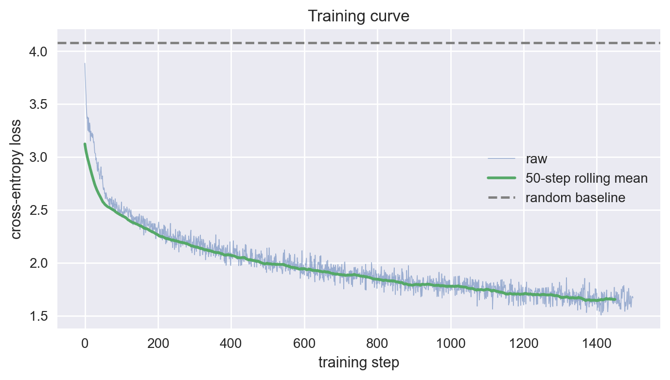
print(f"Initial loss = {initial_loss:.3f}  (random baseline = {np.log(vocab_size):.3f})")

Compilation took 3.5s
Initial loss = 4.078  (random baseline = 4.078)

BATCH_SIZE = 32
N_STEPS = 1500
LOG_EVERY = 100

losses = []
t0 = time.time()
for step in range(N_STEPS):
    x_b, y_b = get_batch(rng_np, BATCH_SIZE, cfg.block_size)
    losses.append(float(train_step(x_b, y_b)))
    if step % LOG_EVERY == 0 or step == N_STEPS - 1:
        recent = np.mean(losses[-LOG_EVERY:])
        print(f"step {step:>4d}  recent-mean loss = {recent:.3f}")
print(f"\nTotal training time: {time.time() - t0:.1f}s")

step    0  recent-mean loss = 3.886
step  100  recent-mean loss = 2.835
step  200  recent-mean loss = 2.398
step  300  recent-mean loss = 2.234
step  400  recent-mean loss = 2.129
step  500  recent-mean loss = 2.050
step  600  recent-mean loss = 1.984
step  700  recent-mean loss = 1.930
step  800  recent-mean loss = 1.884
step  900  recent-mean loss = 1.833
step 1000  recent-mean loss = 1.793
step 1100  recent-mean loss = 1.770
step 1200  recent-mean loss = 1.728
step 1300  recent-mean loss = 1.705
step 1400  recent-mean loss = 1.674
step 1499  recent-mean loss = 1.650

Total training time: 32.3s

fig, ax = plt.subplots(figsize=(8, 4))
ax.plot(losses, lw=0.6, alpha=0.5, label="raw")
win = 50
ax.plot(
    np.arange(len(losses) - win + 1),
    np.convolve(losses, np.ones(win) / win, mode="valid"),
    lw=2, label=f"{win}-step rolling mean",
)
ax.axhline(np.log(vocab_size), color="grey", ls="--", label="random baseline")
ax.set_xlabel("training step")
ax.set_ylabel("cross-entropy loss")
ax.legend()
ax.set_title("Training curve");

Sampling — the autoregressive loop lives inside pytensor.scan

For inference we feed the model a context window and sample the next character from the predicted distribution over the vocabulary. PyTensor lets us push the entire autoregressive loop into the compiled graph with pytensor.scan: every forward pass, every categorical draw, all the context-window bookkeeping becomes a single C/Numba call. We use ptx.random.shared_rng so the RNG state advances inside the compiled function — each call returns an independent draw. This pattern matches the one in the scan tutorial.

We keep the context window and the categorical sampling as xtensor ops: that way the sliding window is a named-dim concat rather than positional pt.concatenate, and categorical consumes a probs xtensor with a vocab core dim. pytensor.scan itself only carries plain tensor variables across iterations, so we cross the xtensor↔tensor boundary in four places: convert to tensor before passing into the scan, back to xtensor at the top of the body, back to tensor before returning, and back to xtensor as soon as we get the scan outputs out.

We also turn this into a while-scan: pytensor.scan accepts a (outputs, until(cond)) return from the body and stops as soon as cond becomes true. Here we stop on the first newline — Tiny Shakespeare uses \n as a hard break between speakers — capped by n_new_sym as a safety net.

from pytensor.scan import until

EOS_ID = stoi["\n"]
rng_sym = ptx.random.shared_rng(seed=2026, name="rng_sample")


def gen_step(context_t, rng):
    """One generation step inside the scan loop.

    `context_t` arrives as a length-`block_size` int64 *tensor* — scan only
    carries tensor variables across iterations — and we immediately wrap it
    as an xtensor with a `time` dim. The forward pass is tensor-native, so
    we dip back to tensor land for that single call, then go back to
    xtensor for the sample + window slide.
    """
    context = ptx.as_xtensor(context_t, dims=("time",))
    assert context.dims == ("time",)

    logits_step = ptx.as_xtensor(
        forward(context_t[None, :], params, cfg)[0, -1], dims=("vocab",)
    )
    probs_step = ptx.math.softmax(logits_step, dim="vocab")
    next_rng, next_tok = rng.categorical(probs_step, core_dims="vocab")
    assert next_tok.dims == ()

    new_context = ptx.concat(
        [context.isel(time=slice(1, None)), next_tok.expand_dims("time")],
        dim="time",
    )
    assert new_context.dims == ("time",)

    return (
        [new_context.values, next_tok.values, next_rng],
        until(pt.eq(next_tok.values, EOS_ID)),
    )


init_ctx_x = ptx.xtensor(
    "init_ctx", dims=("time",), shape=(cfg.block_size,), dtype="int64"
)
n_new_sym = pt.iscalar("n_new")

ctx_seq_t, tok_seq_t, rng_final = pytensor.scan(
    fn=gen_step,
    outputs_info=[init_ctx_x.values, None, rng_sym],
    n_steps=n_new_sym,
    return_updates=False,
)
tok_seq = ptx.as_xtensor(tok_seq_t, dims=("step",))
assert tok_seq.dims == ("step",)

generate_fn = pytensor.function(
    [init_ctx_x, n_new_sym],
    tok_seq.values,
    updates={rng_sym: rng_final},
)


def generate(prompt: str, n_new_tokens: int = 400) -> str:
    """Run autoregressive generation. The Python wrapper only handles text ↔ ids;
    every forward pass and every sample lives inside the compiled scan, which
    stops early at the first newline or after ``n_new_tokens`` steps.
    """
    ids = list(encode(prompt)) or [EOS_ID]
    init_ctx = np.full(cfg.block_size, EOS_ID, dtype="int64")
    init_ctx[-len(ids):] = ids[-cfg.block_size:]
    sampled = generate_fn(init_ctx, n_new_tokens)
    return prompt + decode(sampled)


print(generate("ROMEO:\n", n_new_tokens=400))

ROMEO:
He have shut thing disp: eat fitorer, which bee spose!

Scaling up: a deeper model on more data

The sections above used a 50 K-character slice and a small 2-layer model. Now we double both and train a 4-layer transformer on a 100 K-character slice (and double block_size), still on the default Numba backend. We then compare the two models head-to-head on a held-out slice of Shakespeare that neither has seen — the training losses on their own are not directly comparable because the corpora, vocabularies, and context windows differ.

Re-tokenize a 100 K-character slice and rebuild the model

We use a fresh Config and a freshly initialised parameter dict so this section is independent of everything above.

text_full = full_text[:100_000]
chars_full = sorted(set(text_full))
vocab_size_full = len(chars_full)
stoi_full = {c: i for i, c in enumerate(chars_full)}
itos_full = {i: c for i, c in enumerate(chars_full)}
data_full = np.array([stoi_full[c] for c in text_full], dtype="int64")

cfg_full = Config(
    vocab_size=vocab_size_full,
    block_size=64,
    n_embd=64,
    n_head=4,
    n_layer=4,
)
print(f"corpus slice: {len(data_full):,} chars, vocab: {vocab_size_full}")
print(f"cfg_full    : {cfg_full}")

init_arrays_full = init_params(cfg_full, np.random.default_rng(7))
print(f"params      : {sum(a.size for a in init_arrays_full.values()):,}")

corpus slice: 100,000 chars, vocab: 61
cfg_full    : Config(vocab_size=61, block_size=64, n_embd=64, n_head=4, n_layer=4)
params      : 205,760

Compile a fresh train_step and train

We wrap the now-familiar pattern — fresh shared params, symbolic loss, lower the xtensor sub-graph, pytensor.grad, Adam updates, compile — into a small helper so this section reads top-to-bottom.

def build_train_step(cfg, init_arrays, *, lr=3e-3):
    p = {n: pytensor.shared(arr.copy(), name=n) for n, arr in init_arrays.items()}
    X = pt.tensor("X", shape=(None, cfg.block_size), dtype="int64")
    Y = pt.tensor("Y", shape=(None, cfg.block_size), dtype="int64")
    logits = forward(X, p, cfg)
    log_probs = pt.special.log_softmax(logits, axis=-1)
    bidx = pt.arange(X.shape[0])[:, None]
    tidx = pt.arange(X.shape[1])[None, :]
    loss = (-log_probs[bidx, tidx, Y]).mean()
    # Lower xtensor ops before grad (see the smaller-model section above).
    loss = rewrite_graph(loss, include=("lower_xtensor",))
    grads = pytensor.grad(loss, list(p.values()))
    upd = adam_updates(list(p.values()), grads, lr=lr)
    t0 = time.time()
    fn = pytensor.function([X, Y], loss, updates=upd)
    return fn, p, time.time() - t0

BATCH_FULL = 32
N_STEPS_FULL = 1500

train_step_full, params_full, ct_numba = build_train_step(cfg_full, init_arrays_full)
print(f"Compilation took {ct_numba:.1f}s")

Compilation took 10.3s

rng_full = np.random.default_rng(123)
losses_full: list[float] = []
t0 = time.time()
for step in range(N_STEPS_FULL):
    starts = rng_full.integers(0, len(data_full) - cfg_full.block_size - 1, size=BATCH_FULL)
    xb = np.stack([data_full[s : s + cfg_full.block_size] for s in starts])
    yb = np.stack([data_full[s + 1 : s + 1 + cfg_full.block_size] for s in starts])
    losses_full.append(float(train_step_full(xb, yb)))
    if step % 100 == 0 or step == N_STEPS_FULL - 1:
        print(f"step {step:>4d}  recent-mean loss = {np.mean(losses_full[-100:]):.3f}")
print(f"\nTotal training time: {time.time() - t0:.1f}s")

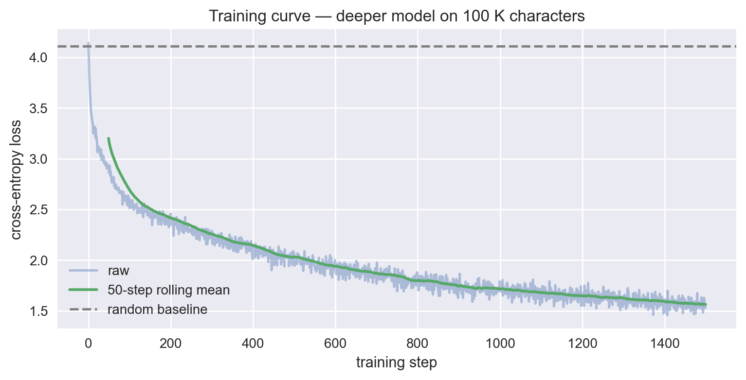
step    0  recent-mean loss = 4.141
step  100  recent-mean loss = 2.934
step  200  recent-mean loss = 2.462
step  300  recent-mean loss = 2.297
step  400  recent-mean loss = 2.163
step  500  recent-mean loss = 2.051
step  600  recent-mean loss = 1.962
step  700  recent-mean loss = 1.884
step  800  recent-mean loss = 1.822
step  900  recent-mean loss = 1.763
step 1000  recent-mean loss = 1.722
step 1100  recent-mean loss = 1.688
step 1200  recent-mean loss = 1.658
step 1300  recent-mean loss = 1.628
step 1400  recent-mean loss = 1.598
step 1499  recent-mean loss = 1.569

Total training time: 185.1s

fig, ax = plt.subplots(figsize=(9, 4))
ax.plot(losses_full, alpha=0.4, label="raw")
rolling = np.convolve(losses_full, np.ones(50) / 50, mode="valid")
ax.plot(np.arange(len(rolling)) + 49, rolling, lw=2, label="50-step rolling mean")
ax.axhline(np.log(cfg_full.vocab_size), ls="--", color="gray", label="random baseline")
ax.set_xlabel("training step")
ax.set_ylabel("cross-entropy loss")
ax.set_title("Training curve — deeper model on 100 K characters")
ax.legend()
plt.show()

A fair side-by-side: held-out perplexity

The two training losses (≈ 1.65 vs ≈ 1.57) aren’t directly comparable. The models saw different corpus slices (50 K vs 100 K characters), have different vocabularies (59 vs 61), and — most importantly — a different block_size (32 vs 64). Doubling the context window alone tends to drive per-token cross-entropy down, even at equal model quality.

To get an honest comparison we evaluate both models on the same 10 K-character slice that neither of them saw during training (full_text[100_000:110_000]). For the small model we simply skip the handful of characters that aren’t in its vocabulary.

def build_eval_fn(cfg, params_dict):
    """Compile a forward + cross-entropy function that reads from the shared params."""
    X = pt.tensor("X_eval", shape=(None, cfg.block_size), dtype="int64")
    Y = pt.tensor("Y_eval", shape=(None, cfg.block_size), dtype="int64")
    log_probs = pt.special.log_softmax(forward(X, params_dict, cfg), axis=-1)
    bidx = pt.arange(X.shape[0])[:, None]
    tidx = pt.arange(X.shape[1])[None, :]
    loss = (-log_probs[bidx, tidx, Y]).mean()
    loss = rewrite_graph(loss, include=("lower_xtensor",))
    return pytensor.function([X, Y], loss)


def held_out_loss(eval_fn, cfg, stoi_local, holdout_text):
    """Mean per-token cross-entropy over non-overlapping windows of `holdout_text`.
    Characters absent from `stoi_local` are skipped (vocabularies can differ slightly)."""
    ids = np.array([stoi_local[c] for c in holdout_text if c in stoi_local], dtype="int64")
    starts = np.arange(0, len(ids) - cfg.block_size - 1, cfg.block_size)
    total, n = 0.0, 0
    for i in range(0, len(starts), 64):
        batch = starts[i : i + 64]
        xb = np.stack([ids[s : s + cfg.block_size] for s in batch])
        yb = np.stack([ids[s + 1 : s + 1 + cfg.block_size] for s in batch])
        total += float(eval_fn(xb, yb)) * len(batch)
        n += len(batch)
    return total / n


holdout_text = full_text[100_000:110_000]
L_small = held_out_loss(build_eval_fn(cfg, params),           cfg,      stoi,      holdout_text)
L_full  = held_out_loss(build_eval_fn(cfg_full, params_full), cfg_full, stoi_full, holdout_text)

print(f"held-out CE  (small, 2-layer, block 32): {L_small:.3f}  ppl = {np.exp(L_small):.2f}")
print(f"held-out CE  (large, 4-layer, block 64): {L_full :.3f}  ppl = {np.exp(L_full ):.2f}")

held-out CE  (small, 2-layer, block 32): 1.841  ppl = 6.31
held-out CE  (large, 4-layer, block 64): 1.738  ppl = 5.69

A sample from the deeper model

On held-out text the deeper model is genuinely better — about 0.10 nats per character lower cross-entropy, or ~10% lower perplexity (5.69 vs 6.31). At this scale and training budget that is not enough to make the samples look coherent: both models still produce Shakespearean gibberish at the word level. What you can see in the sample below is firmer speaker-name structure and slightly more believable rhythm. We reuse the same pytensor.scan generator pattern — the entire autoregressive loop still lives inside one compiled call.

EOS_ID_FULL = stoi_full["\n"]
rng_full_sym = ptx.random.shared_rng(seed=2027, name="rng_full")


def gen_step_full(context_t, rng):
    context = ptx.as_xtensor(context_t, dims=("time",))
    logits_step = ptx.as_xtensor(
        forward(context_t[None, :], params_full, cfg_full)[0, -1], dims=("vocab",)
    )
    probs_step = ptx.math.softmax(logits_step, dim="vocab")
    next_rng, next_tok = rng.categorical(probs_step, core_dims="vocab")
    new_context = ptx.concat(
        [context.isel(time=slice(1, None)), next_tok.expand_dims("time")],
        dim="time",
    )
    return (
        [new_context.values, next_tok.values, next_rng],
        until(pt.eq(next_tok.values, EOS_ID_FULL)),
    )


init_ctx_full = ptx.xtensor(
    "init_ctx_full", dims=("time",), shape=(cfg_full.block_size,), dtype="int64"
)
n_new_full = pt.iscalar("n_new_full")

_, tok_seq_full_t, rng_final_full = pytensor.scan(
    fn=gen_step_full,
    outputs_info=[init_ctx_full.values, None, rng_full_sym],
    n_steps=n_new_full,
    return_updates=False,
)
tok_seq_full = ptx.as_xtensor(tok_seq_full_t, dims=("step",))

generate_full_fn = pytensor.function(
    [init_ctx_full, n_new_full],
    tok_seq_full.values,
    updates={rng_full_sym: rng_final_full},
)


def generate_full(prompt: str, n_new_tokens: int = 400) -> str:
    ids = list(np.array([stoi_full[c] for c in prompt], dtype="int64")) or [EOS_ID_FULL]
    init_ctx = np.full(cfg_full.block_size, EOS_ID_FULL, dtype="int64")
    init_ctx[-len(ids):] = ids[-cfg_full.block_size:]
    sampled = generate_full_fn(init_ctx, n_new_tokens)
    return prompt + "".join(itos_full[int(i)] for i in sampled)

print(generate_full("ROMEO:\n", n_new_tokens=400))

ROMEO:
But be teak of the thus.

Takeaways

• A full decoder-only transformer — embeddings, multi-head causal attention, MLP, layernorm, tied softmax head, cross-entropy loss, and Adam — fits in roughly 100 lines of PyTensor. No custom Op, no backend-specific code.

• pytensor.xtensor named dimensions turned the trickiest part of the model (multi-head attention) into self-documenting code. The named-dim sub-graph is lowered to plain tensor ops at compile time — we just had to call rewrite_graph(loss, include=("lower_xtensor",)) once before pytensor.grad so the gradient pass walks the lowered graph.

• pytensor.grad gave us back-propagation through the entire stack as a new symbolic graph. We optimised that graph and compiled it into a single C/Numba train_step.

• pytensor.shared plus updates= made Adam a 15-line helper. Optimizer state lives next to the parameters in the graph, not in Python.

• pytensor.scan let us push autoregressive generation entirely inside the compiled graph — the Python wrapper only translates between text and ids; every forward pass and every categorical draw lives inside one C/Numba call.

Where to go from here

• Swap mode="NUMBA" (default) for mode="JAX" to train on a GPU/TPU.

• Replace tanh with a real GELU and try a longer training run on the full 1.1 M-character corpus.

• Use pytensor.dprint(train_step) to inspect the optimised post-rewrite graph and see how many ops PyTensor’s rewriter fused away.

Authors

• Authored by the PyTensor developers in May 2026.

Watermark

%load_ext watermark
%watermark -n -u -v -iv -w -p pytensor

Last updated: Tue, 16 Jun 2026

Python implementation: CPython
Python version       : 3.14.4
IPython version      : 9.13.0

pytensor: 3.0.5+30.g1bb3ee02f

matplotlib: 3.10.9
numpy     : 2.4.3
pytensor  : 3.0.5+30.g1bb3ee02f

Watermark: 2.6.0

License notice

All the notebooks in this example gallery are provided under a 3-Clause BSD License which allows modification, and redistribution for any use provided the copyright and license notices are preserved.

Citing Pytensor Examples

To cite this notebook, please use the suggested citation below.

Important

Many notebooks are adapted from other sources: blogs, books… In such cases you should cite the original source as well.

Also remember to cite the relevant libraries used by your code.

Here is an example citation template in bibtex:

@incollection{citekey,
  author    = "<notebook authors, see above>",
  title     = "<notebook title>",
  editor    = "Pytensor Team",
  booktitle = "Pytensor Examples",
}

which once rendered could look like: