Derivatives in PyTensor#

Computing Gradients#

Now let’s use PyTensor for a slightly more sophisticated task: create a function which computes the derivative of some expression y with respect to its parameter x. To do this we will use the macro pt.grad. For instance, we can compute the gradient of \(x^2\) with respect to \(x\). Note that: \(d(x^2)/dx = 2 \cdot x\).

Here is the code to compute this gradient:

>>> import numpy
>>> import pytensor
>>> import pytensor.tensor as pt
>>> from pytensor import pp
>>> x = pt.dscalar('x')
>>> y = x ** 2
>>> gy = pt.grad(y, x)
>>> pp(gy)  # print out the gradient prior to optimization
'((fill((x ** TensorConstant{2}), TensorConstant{1.0}) * TensorConstant{2}) * (x ** (TensorConstant{2} - TensorConstant{1})))'
>>> f = pytensor.function([x], gy)
>>> f(4)
array(8.0)
>>> numpy.allclose(f(94.2), 188.4)
True

In this example, we can see from pp(gy) that we are computing the correct symbolic gradient. fill((x**2), 1.0) means to make a matrix of the same shape as x**2 and fill it with 1.0.

Note

PyTensor’s rewrites simplify the symbolic gradient expression. You can see this by digging inside the internal properties of the compiled function.

pp(f.maker.fgraph.outputs[0])
'(2.0 * x)'

After rewriting, there is only one Apply node left in the graph.

We can also compute the gradient of complex expressions such as the logistic function defined above. It turns out that the derivative of the logistic is: \(ds(x)/dx = s(x) \cdot (1 - s(x))\).

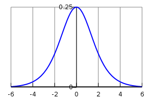
../_images/dlogistic.png — A plot of the gradient of the logistic function, with \(x\) on the x-axis and \(ds(x)/dx\) on the \(y\)-axis.#

>>> x = pt.dmatrix('x')
>>> s = pt.sum(1 / (1 + pt.exp(-x)))
>>> gs = pt.grad(s, x)
>>> dlogistic = pytensor.function([x], gs)
>>> dlogistic([[0, 1], [-1, -2]])
array([[ 0.25      ,  0.19661193],
       [ 0.19661193,  0.10499359]])

In general, for any scalar expression s, pt.grad(s, w) provides the PyTensor expression for computing \(\frac{\partial s}{\partial w}\). In this way PyTensor can be used for doing efficient symbolic differentiation (as the expression returned by pt.grad will be optimized during compilation), even for function with many inputs. (see automatic differentiation for a description of symbolic differentiation).

Note

The second argument of pt.grad can be a list, in which case the output is also a list. The order in both lists is important: element i of the output list is the gradient of the first argument of pt.grad with respect to the i-th element of the list given as second argument. The first argument of pt.grad has to be a scalar (a tensor of size 1). For more information on the semantics of the arguments of pt.grad and details about the implementation, see this section of the library.

Additional information on the inner workings of differentiation may also be found in the more advanced tutorial Extending PyTensor.

Computing the Jacobian#

In PyTensor’s parlance, the term Jacobian designates the tensor comprising the first partial derivatives of the output of a function with respect to its inputs. (This is a generalization of to the so-called Jacobian matrix in Mathematics.) PyTensor implements the pytensor.gradient.jacobian() macro that does all that is needed to compute the Jacobian. The following text explains how to do it manually.

In order to manually compute the Jacobian of some function y with respect to some parameter x we need to use scan. What we do is to loop over the entries in y and compute the gradient of y[i] with respect to x.

Note

scan is a generic op in PyTensor that allows writing in a symbolic manner all kinds of recurrent equations. While creating symbolic loops (and optimizing them for performance) is a hard task, effort is being done for improving the performance of scan. We shall return to scan later in this tutorial.

>>> import pytensor
>>> import pytensor.tensor as pt
>>> x = pt.dvector('x')
>>> y = x ** 2
>>> J, updates = pytensor.scan(lambda i, y, x : pt.grad(y[i], x), sequences=pt.arange(y.shape[0]), non_sequences=[y, x])
>>> f = pytensor.function([x], J, updates=updates)
>>> f([4, 4])
array([[ 8.,  0.],
       [ 0.,  8.]])

What we do in this code is to generate a sequence of integers from 0 to y.shape[0] using pt.arange. Then we loop through this sequence, and at each step, we compute the gradient of element y[i] with respect to x. scan automatically concatenates all these rows, generating a matrix which corresponds to the Jacobian.

Note

There are some pitfalls to be aware of regarding pt.grad. One of them is that you cannot re-write the above expression of the Jacobian as pytensor.scan(lambda y_i,x: pt.grad(y_i,x), sequences=y, non_sequences=x), even though from the documentation of scan this seems possible. The reason is that y_i will not be a function of x anymore, while y[i] still is.

Computing the Hessian#

In PyTensor, the term Hessian has the usual mathematical meaning: It is the matrix comprising the second order partial derivative of a function with scalar output and vector input. PyTensor implements pytensor.gradient.hessian() macro that does all that is needed to compute the Hessian. The following text explains how to do it manually.

You can compute the Hessian manually similarly to the Jacobian. The only difference is that now, instead of computing the Jacobian of some expression y, we compute the Jacobian of pt.grad(cost,x), where cost is some scalar.

>>> x = pt.dvector('x')
>>> y = x ** 2
>>> cost = y.sum()
>>> gy = pt.grad(cost, x)
>>> H, updates = pytensor.scan(lambda i, gy,x : pt.grad(gy[i], x), sequences=pt.arange(gy.shape[0]), non_sequences=[gy, x])
>>> f = pytensor.function([x], H, updates=updates)
>>> f([4, 4])
array([[ 2.,  0.],
       [ 0.,  2.]])

Jacobian times a Vector#

Sometimes we can express the algorithm in terms of Jacobians times vectors, or vectors times Jacobians. Compared to evaluating the Jacobian and then doing the product, there are methods that compute the desired results while avoiding actual evaluation of the Jacobian. This can bring about significant performance gains. A description of one such algorithm can be found here:

Barak A. Pearlmutter, “Fast Exact Multiplication by the Hessian”, Neural Computation, 1994

While in principle we would want PyTensor to identify these patterns automatically for us, in practice, implementing such optimizations in a generic manner is extremely difficult. Therefore, we provide special functions dedicated to these tasks.

R-operator#

The R operator is built to evaluate the product between a Jacobian and a vector, namely \(\frac{\partial f(x)}{\partial x} v\). The formulation can be extended even for \(x\) being a matrix, or a tensor in general, case in which also the Jacobian becomes a tensor and the product becomes some kind of tensor product. Because in practice we end up needing to compute such expressions in terms of weight matrices, PyTensor supports this more generic form of the operation. In order to evaluate the R-operation of expression y, with respect to x, multiplying the Jacobian with V you need to do something similar to this:

>>> W = pt.dmatrix('W')
>>> V = pt.dmatrix('V')
>>> x = pt.dvector('x')
>>> y = pt.dot(x, W)
>>> JV = pytensor.gradient.Rop(y, W, V)
>>> f = pytensor.function([W, V, x], JV)
>>> f([[1, 1], [1, 1]], [[2, 2], [2, 2]], [0,1])
array([ 2.,  2.])

List of Op that implement Rop.

L-operator#

In similitude to the R-operator, the L-operator would compute a row vector times the Jacobian. The mathematical formula would be \(v \frac{\partial f(x)}{\partial x}\). The L-operator is also supported for generic tensors (not only for vectors). Similarly, it can be implemented as follows:

>>> W = pt.dmatrix('W')
>>> v = pt.dvector('v')
>>> x = pt.dvector('x')
>>> y = pt.dot(x, W)
>>> VJ = pytensor.gradient.Lop(y, W, v)
>>> f = pytensor.function([v,x], VJ)
>>> f([2, 2], [0, 1])
array([[ 0.,  0.],
       [ 2.,  2.]])

Note

v, the point of evaluation, differs between the L-operator and the R-operator. For the L-operator, the point of evaluation needs to have the same shape as the output, whereas for the R-operator this point should have the same shape as the input parameter. Furthermore, the results of these two operations differ. The result of the L-operator is of the same shape as the input parameter, while the result of the R-operator has a shape similar to that of the output.

List of op with r op support.

Hessian times a Vector#

If you need to compute the Hessian times a vector, you can make use of the above-defined operators to do it more efficiently than actually computing the exact Hessian and then performing the product. Due to the symmetry of the Hessian matrix, you have two options that will give you the same result, though these options might exhibit differing performances. Hence, we suggest profiling the methods before using either one of the two:

>>> x = pt.dvector('x')
>>> v = pt.dvector('v')
>>> y = pt.sum(x ** 2)
>>> gy = pt.grad(y, x)
>>> vH = pt.grad(pt.sum(gy * v), x)
>>> f = pytensor.function([x, v], vH)
>>> f([4, 4], [2, 2])
array([ 4.,  4.])

or, making use of the R-operator:

>>> x = pt.dvector('x')
>>> v = pt.dvector('v')
>>> y = pt.sum(x ** 2)
>>> gy = pt.grad(y, x)
>>> Hv = pytensor.gradient.Rop(gy, x, v)
>>> f = pytensor.function([x, v], Hv)
>>> f([4, 4], [2, 2])
array([ 4.,  4.])

Final Pointers#

The grad function works symbolically: it receives and returns PyTensor variables.
grad can be compared to a macro since it can be applied repeatedly.
Scalar costs only can be directly handled by grad. Arrays are handled through repeated applications.
Built-in functions allow to compute efficiently vector times Jacobian and vector times Hessian.
Work is in progress on the optimizations required to compute efficiently the full Jacobian and the Hessian matrix as well as the Jacobian times vector.